
In this exercise, the support reactions of a symmetrical multi-span beam supported on three columns are calculated. Here is an online calculator here for calculating asymmetrical multi-span beams.
Task
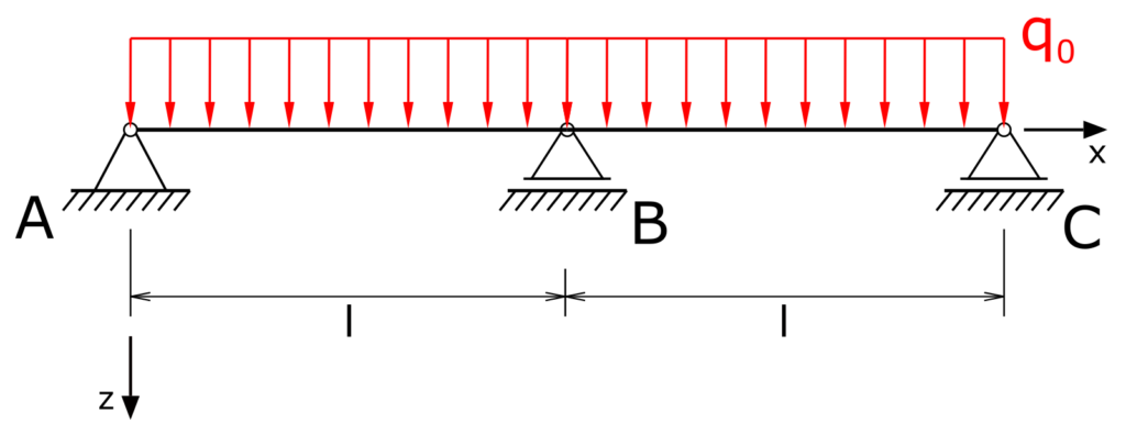
A continuous beam on a fixed bearing and two floating bearings (multi-span beam) with the symmetrical column width l is loaded by a line load q0. How big are the bearing loads?
Solution
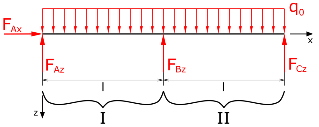
In the first step, the equations for the bearing reactions are determined. For the subsequent determination of the internal forces, the beam is divided into two areas. The horizontal forces are not considered further in the following equations, since they are obviously zero. Left turning moments are positive.
Determination of the bearing loads
The sum of forces in z-direction is
\[ \tag{1} \sum F_z = 0 = -F_{Az} - F_{Bz} - F_{Cz} + \int_0^{2l}{q_0dx} \]
\[ \tag{2} 0 = -F_{Az} - F_{Bz} - F_{Cz} + 2 \cdot q_0 \cdot l \]
The sum of moments at A
\[ \tag{3} \sum M(A) = 0 = F_{Bz} \cdot l + 2 \cdot F_{Cz} \cdot l - \int_0^{2l}{q_0xdx} \]
\[ \tag{4} 0 = F_{Bz} \cdot l + 2 \cdot F_{Cz} \cdot l - 2 \cdot q_0 \cdot l^2 \]
This results in a system of equations with 2 equations but 3 unknowns. The next step is to determine the internal forces in the two sections I and II. In order to be able to integrate the function of the line load from 0 to x, it is formulated as a function of the auxiliary coordinate ξ. Normal forces are denoted by N, transverse forces by Q and bending moments by Mb.
Determination of the internal forces
Section I
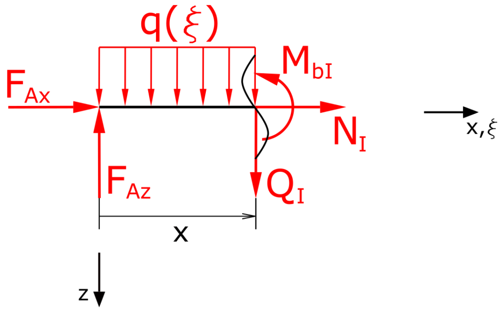
The sum of forces in z-direction is
\[ \tag{5} \sum F_z = 0 = -F_{Az} + Q_I + \int_0^{x}{q_0d \xi} \]
\[ \tag{6} 0 = -F_{Az} + Q_I + q_0 \cdot x \]
The sum of moments at x is
\[ \tag{7} \sum M(x) = 0 = \int_0^{x}{q_0 \xi d \xi} - F_{Az} \cdot x + M_{bI} \]
\[ \tag{8} 0 = \frac{1}{2} q_0 x^2 - F_{Az} \cdot x + M_{bI} \]
Section II
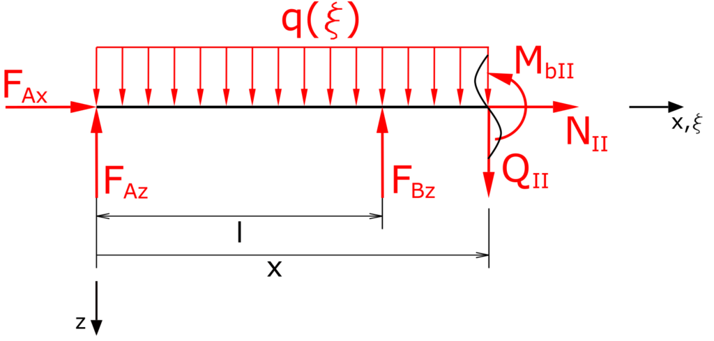
The sum of forces in z-direction is
\[ \tag{9} \sum F_z = 0 = -F_{Az} -F_{Bz}+ Q_{II} + \int_0^{x}{q_0d \xi} \]
\[ \tag{10} 0 = -F_{Az} -F_{Bz}+ Q_{II} + q_0 x \]
The sum of moments at x
\[ \tag{11} \sum M(x) = 0 = \int_0^{x}{q_0 \xi d \xi} - F_{Az} \cdot x - F_{Az} \cdot (x-l) + M_{bII} \]
\[ \tag{12} 0 = \frac{1}{2} q_0 x^2 - F_{Az} \cdot x - F_{Bz} \cdot (x-l) + M_{bII} \]
Next, the functions of the bending lines are calculated.
Bending lines
The function of the bending line is designated as w, or the first derivative as w' and the second derivative as w''. The modulus of elasticity is E (Young's modulus) and the area moment of inertia is I.
Section I
\[ \tag{13} M_{bI} = -\frac{{q_0} {{x}^{2}}-2 {F_{\mathit{Az}}} x}{2} \]
\[ \tag{14} w''_I = - \frac{1}{E \cdot I} M_{bI} \]
\[ \tag{15} w''_I = \frac{{q_0} {{x}^{2}}-2 {F_{\mathit{Az}}} x}{2 E I} \]
\[ \tag{16} w'_I = \frac{\frac{{q_0} {{x}^{3}}}{3}-{F_{\mathit{Az}}} {{x}^{2}}}{2 E I}+\mathit{ c_1} \]
\[ \tag{17} w_I = \frac{\frac{{q_0} {{x}^{4}}}{12}-\frac{{F_{\mathit{Az}}} {{x}^{3}}}{3}}{2 E I}+\mathit{ c_1} x+\mathit{ c_2} \]
Section II
\[ \tag{18} M_{bII} = -\frac{{q_o} {{x}^{2}}+\left( -2 {F_{\mathit{Bz}}}-2 {F_{\mathit{Az}}}\right) x+2 {F_{\mathit{Bz}}} l}{2}\]
\[ \tag{19} w''_{II} = - \frac{1}{E \cdot I} M_{bII} \]
\[ \tag{20} w''_{II} = \frac{{q_o} {{x}^{2}}+\left( -2 {F_{\mathit{Bz}}}-2 {F_{\mathit{Az}}}\right) x+2 {F_{\mathit{Bz}}} l}{2 E I} \]
\[ \tag{21} w'_{II} = \frac{\frac{{q_o} {{x}^{3}}}{3}+\frac{\left( -2 {F_{\mathit{Bz}}}-2 {F_{\mathit{Az}}}\right) {{x}^{2}}}{2}+2 {F_{\mathit{Bz}}} l x}{2 E I}+\mathit{ c_3} \]
\[ \tag{22} w_{II} = \frac{\frac{{q_o} {{x}^{4}}}{12}+\frac{\left( -2 {F_{\mathit{Bz}}}-2 {F_{\mathit{Az}}}\right) {{x}^{3}}}{6}+{F_{\mathit{Bz}}} l\, {{x}^{2}}}{2 E I}+\mathit{ c_3} x+\mathit{ c_4} \]
The constants of integration are determined via the boundary and transition conditions.
Boundary and transition conditions
The deflection at the point x = 0 is equal to zero.
\[ \tag{23} 0=\mathit{c_2} \]
The deflection at the point x = l is zero. This condition can be used for both bending lines.
\[ \tag{24} \frac{\frac{{{l}^{4}}\, {q_0}}{12}-\frac{{F_{\mathit{Az}}} {{l}^{3}}}{3}}{2 E I}+\mathit{c_1} l = 0\]
\[ \tag{25} \frac{\frac{{{l}^{4}}\, {q_o}}{12}+{F_{\mathit{Bz}}} {{l}^{3}}+\frac{\left( -2 {F_{\mathit{Bz}}}-2 {F_{\mathit{Az}}}\right) {{l}^{3}}}{6}}{2 E I}+\mathit{ c_3} l+\mathit{ c_4}=0\]
The deflection at the point x = 2l is zero.
\[ \tag{26} \frac{\frac{4 {{l}^{4}}\, {q_o}}{3}+4 {F_{\mathit{Bz}}} {{l}^{3}}+\frac{4 \left( -2 {F_{\mathit{Bz}}}-2 {F_{\mathit{Az}}}\right) {{l}^{3}}}{3}}{2 E I}+2 \mathit{ c_3} l+\mathit{ c_4} \]
Both bending lines have the same angle at the point x = 1.
\[ \tag{27} \frac{\frac{{{l}^{3}}\, {q_0}}{3}-{F_{\mathit{Az}}} {{l}^{2}}}{2 E I}+\mathit{ c_1} = \frac{\frac{{{l}^{3}}\, {q_o}}{3}+2 {F_{\mathit{Bz}}} {{l}^{2}}+\frac{\left( -2 {F_{\mathit{Bz}}}-2 {F_{\mathit{Az}}}\right) {{l}^{2}}}{2}}{2 E I}+\mathit{ c_3} \]
There are now sufficient equations to be able to solve the unknowns.
\[ \tag{28} \mathit{ c_1}=\frac{11 {{l}^{3}}\, {q_o}-9 {{l}^{3}}\, {q_0}}{96 E I} \]
\[ \tag{29} c_2 = 0 \]
\[ \tag{30} \mathit{ c_3}=\frac{61 {{l}^{3}}\, {q_o}-119 {{l}^{3}}\, {q_0}}{96 E I} \]
\[ \tag{31} \mathit{ c_4}=-\frac{5 {{l}^{4}}\, {q_o}-15 {{l}^{4}}\, {q_0}}{48 E I} \]
\[ \tag{32} {F_{\mathit{Az}}}=\frac{11 l\, {q_o}-5 l\, {q_0}}{16} \]
\[ \tag{33} {F_{\mathit{Bz}}}=-\frac{11 l\, {q_o}-21 l\, {q_0}}{8} \]
\[ \tag{34} {F_{\mathit{Cz}}}=\frac{11 l\, {q_o}-5 l\, {q_0}}{16} \]
And for the sake of completeness
\[ \tag{35} F_{Ax} = 0 \]