Calculation of bearing loads and joint forces

This exercise addresses the following questions:

• How do you calculate joint forces?
• How do I calculate a frame with two fixed bearings?
• What are the different approaches to calculating joint forces?

Task

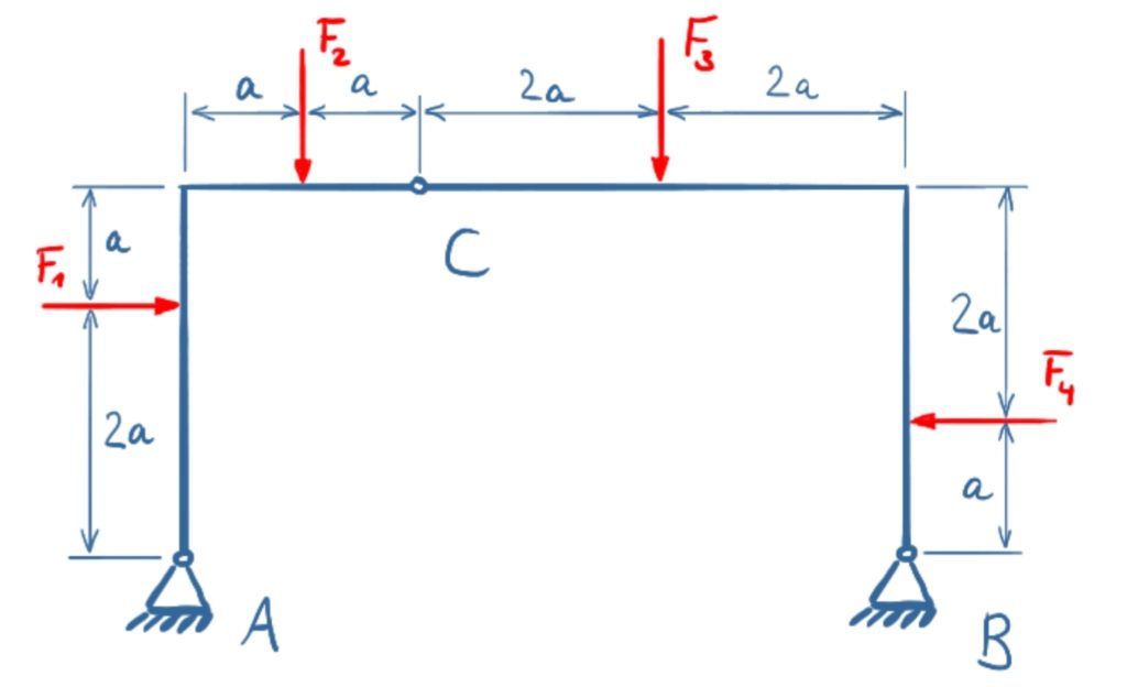
The forces F₁ to F₄ act on a frame with two fixed bearings and a joint. Determine the bearing loads and the forces in joint C!

F₁ = F₄ = 10 kN, F₂ = 30 kN, F₃ = 60 kN, a = 1 m

Solution

The solution can be done in different ways, here two variants are shown:

Solution variant 1 considers both areas to the left and right of the joint separately from the beginning and sets up the corresponding equations.

Solution variant 2 sets up the equilibrium conditions for the entire system as the first step, and then releases the forces of the sub-areas.

Variant 1

The following video is in German language.

Lagerreaktionen und Gelenkkräfte berechnen - Technische Mechanik 1, Übung 22

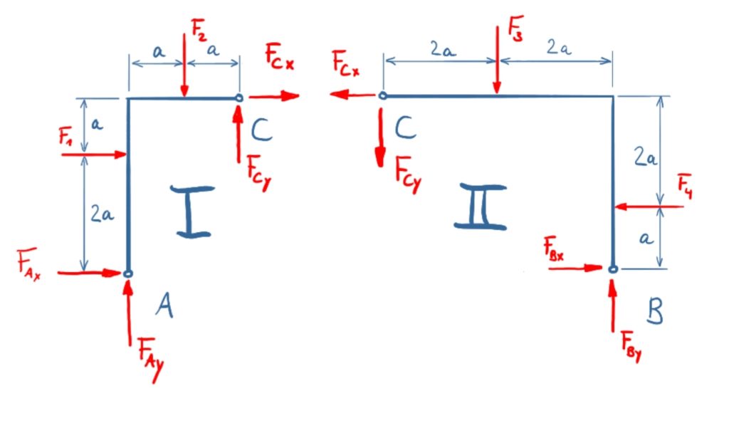
The frame will be divided into two sections to determine the forces.

\[\tag{1} 0={F_{\mathit{Cx}}}+{F_{\mathit{Ax}}}+{F_1}\]

\[\tag{2} 0={F_{\mathit{Cy}}}+{F_{\mathit{Ay}}}-{F_2}\]

\[\tag{4} 0=-{F_{\mathit{Cx}}}+{F_{\mathit{Bx}}}-{F_4}\]

\[\tag{5} 0=-{F_{\mathit{Cy}}}+{F_{\mathit{By}}}-{F_3}\]

\[\tag{7} {F_{\mathit{Ax}}}=-{F_{\mathit{Cx}}}-{F_1}\]

\[\tag{8} {F_{\mathit{Cx}}}=\frac{2 {F_{\mathit{Cy}}}-{F_2}-2 {F_1}}{3}\]

\[\tag{10} {F_{\mathit{Cy}}}=-\frac{3 {F_{\mathit{Cx}}}+{F_4}+2 {F_3}}{4}\]

\[\tag{13} {F_{\mathit{Bx}}}={F_{\mathit{Cx}}}+{F_4}\]

\[\tag{16} {F_{\mathit{By}}}={F_{\mathit{Cy}}}+{F_3}\]

\[\tag{19} {F_{\mathit{Ay}}}={F_2}-{F_{\mathit{Cy}}}\]

\[\tag{27} {F_{\mathit{Ax}}}=15.56 \mathit{kN}\]

\[\tag{28} {F_{\mathit{Ay}}}=43.33 \mathit{kN}\]

\[\tag{29} {F_{\mathit{Bx}}}=-15.56 \mathit{kN}\]

\[\tag{30} {F_{\mathit{By}}}=46.67 \mathit{kN}\]

\[\tag{31} {F_{\mathit{Cx}}}=-25.56 \mathit{kN}\]

\[\tag{32} {F_{\mathit{Cy}}}=-13.33 \mathit{kN}\]

---

Variant 2

This solution is calculated here exclusively with the variables, since the numerical values ​​have already been calculated above.

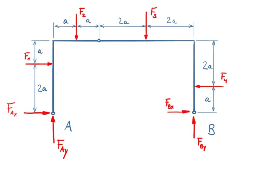
Establishing the balance of forces and moments for the entire system

The vertical support reaction F_By can thus be calculated directly:

F_By is now substituted into equation 1, whereby F_Ay follows.

Next, the balance of forces in the y-direction is set up for section I in order to calculate the joint force F_Cy:

The sum of moments around A leads to F_Cx.

The equilibrium of forces in the x-direction for section I results in the horizontal support reaction in A.:

\[\tag{11} 0={F_{\mathit{Cx}}}+{F_{\mathit{Ax}}}+{F_1}\]

F_Ax is now substituted into equation 2, whereby F_Bx follows.

The second solution leads to the desired results faster!